> For the complete documentation index, see [llms.txt](https://guide.cryosparc.com/llms.txt). Markdown versions of documentation pages are available by appending `.md` to page URLs; this page is available as [Markdown](https://guide.cryosparc.com/the-fsc-and-gold-standard-refinement.md). # The FSC and Gold-Standard Refinement ## Overview Single particle analysis attempts to iteratively estimate some unknown quantity (the 3D volume) from a set of incomplete and noisy observations (the 2D particle images). Problems of this nature are potentially susceptible to overfitting, meaning that noise from the data remains or is amplified in the estimated 3D volume. The Fourier Shell Correlation (FSC) is a measure of correlation between two volumes as a function of signal frequency (Harauz and van Heel, 1986) and can be used in many different ways, for example comparing an experimental 3D density map with a map derived from an atomic model. If two volumes are independently produced from half of the particle images each, the FSC computed between them is known as the gold-standard FSC (GSFSC) and is one way of measuring the degree of overfitting present at each spatial frequency in a map. The GSCFSC tells us how much we can trust the reconstruction at each resolution since the two volumes will have trustable signal in common, while the noise in each map will be different. The GSFSC's trustability estimate can be used to validate the resulting volume. Building on this idea, gold-standard refinement attempts to limit overfitting from building up iteratively by lowpass filtering the 3D reference volume during each image alignment phase of the [Expectation-Maximization](https://guide.cryosparc.com/expectation-maximization-in-cryo-em) algorithm using the GSFSC curve (Scheres and Chen 2012). ## Before Reading This Page {% hint style="info" %} The Fourier transform is a foundational concept for all of signal processing, including cryo-EM. The next section provides a brief overview of the Fourier transform and Fourier space, focusing on the parts which are useful for understanding GS refinement, but it is by no means an exhaustive explanation of the Fourier transform. If the Fourier transform is completely unfamiliar to you, you may find a more thorough review helpful before proceeding. A good starting place might be [this overview from Better Explained](https://betterexplained.com/articles/an-interactive-guide-to-the-fourier-transform/) or this [article from 3blue1brown](https://www.3blue1brown.com/lessons/fourier-transforms). {% endhint %} {% hint style="info" %} This page assumes some familiarity with the Expectation Maximization algorithm in cryo-EM. If you are not familiar with this topic, we recommend you return to this page after reading the [dedicated Expectation Maximization guide page](https://guide.cryosparc.com/expectation-maximization-in-cryo-em). {% endhint %} {% hint style="info" %} Throughout this page examples are typically given in 2D. This is for convenience of display only — the concepts apply equally well to 3D objects like cryo-EM volumes. {% endhint %} ## Overfitting ### Overfitting creates spurious features in aligned averages In single particle analysis, we align particle images to a reference and then update the reference using the newly aligned particle images. This iterative process creates a potential for *overfitting*. A volume is *overfit* when it has detail that is purely an artifact of noise in the particle images; over iterations, overfitting can build up as the artefactual details impact subsequent alignments. This problem is often called “Einstein from noise” in homage to [Richard Henderson’s paper on the topic](https://doi.org/10.1073/pnas.1314449110) demonstrating that you can create an image of anything, including Einstein, from pure noise. We recreate this example here. Consider the following scenario: * The reference (the object that we align the images to) is a high-resolution picture of Albert Einstein. * The images are pure Gaussian noise — they have zero real signal of Einstein. However, as with real cryo-EM datasets, we have no way of knowing that the images are junk — we assume they are noisy images of the reference. When we align all of these images of *random noise* and average them together, we recover an image of Einstein from pure noise.

This result may be surprising — how could we get an image of Einstein by averaging together thousands of images that do not contain any Einstein signal? This process may be easier to understand with a very simple example. Consider the following setup: * our reference and particle images have only 25 pixels * the only allowable poses are rotations by 0, 90, 180, or 270 degrees. No shifts are allowed

The reference has two high-resolution features: single, bright pixels. In the images, on the other hand, some pixels in the noise images are bright and some are dark by pure chance. It is very unlikely that any image, by random chance, has the exact arrangement of dark and light pixels as we see in the reference. When a noise image is aligned to the reference, the best pose tends to line up the brightest pixels in the image with the reference’s bright pixels. When the noise image is in this pose, the sum of the difference between the image and the reference (the pose's *error*) is minimized. This is all that is meant by calling a pose "best" -- it has the lowest error. A single image aligned in this way doesn’t look any more like the reference than it did before alignment. There are dark and light pixels scattered throughout the image. However, as we add more and more images, the bright pixels are always aligned to the same place, while the other pixels may be lighter or may be darker. When we average all of these aligned images together, the bright pixels’ consistent placement produces an average which looks like the reference, even though no image looked like the reference on its own. ### Spurious map features from overfitting The images above were created with only a single iteration of alignment to a reference. In a normal 2D Classification or refinement job, several iterations are performed. Because each subsequent iteration uses the previous iteration’s result as a reference, the overfit noise features can compound and become stronger and stronger. For example, in the first iteration it may be that when all of the noise images were aligned to Einstein, the resulting average looked like Einstein but also had a bright bit of noise somewhere near his face. In the next iteration, this bright stripe might encourage images to put more bright pixels there, making the bright stripe stronger (even though there is no bright stripe in the image themselves or in a true image of Einstein). This problem can create spurious map features even when the images truly are images of the target object, because *all* images have noise. Overfitting is therefore a critical problem in single particle analysis, but it can be mitigated by only presenting alignment algorithms with a lowpass filtered reference at every iteration. ### Lowpass filtering limits overfitting The alignment algorithm was able to create an overfit image because we provided a *high-resolution* reference with fine details. If we lowpass filter the reference before alignment, we still recreate a copy of our input reference. However, because the reference was lowpass filtered, the noise can only be aligned to (and overfit to) low resolution features. Thus, instead of individual locks of Einstein’s hair, we see a light-colored blob:

We can see why by again considering our simple example.

The lowpass filtered reference no longer has single bright pixels. Instead, the bright pixels have spread out to make some regions of the reference darker and some lighter. Thus, when we align the same noise image as before, the optimal pose (i.e., the one with the least error) aligns the darkest pixels to these dark regions of the reference. The light pixels are in a different position, but that doesn’t matter since the reference no longer has bright pixels. In *real images*, the high resolution signal is coupled to the low-resolution signal. If Einstein’s nose (a low-frequency signal) is in the wrong place, the strands of his hair (a high-frequency signal) will be rotated and shifted by the same amount. Aligning one aligns the other. *But pure noise has no such coupling across spatial frequencie*s. The pixel patterns which match Einstein’s hair may be in any position relative to the pixel patterns which match his nose. {% hint style="info" %} **Critical point**. For real signal, the best-fitting pose against a low-resolution reference is very similar to the best-fitting pose against a high-resolution reference. For overfit noise, the pose matching a low-resolution reference may be very different from that matching a high-resolution reference. {% endhint %} Thus, aligning *real images* to a lowpass filtered reference can recreate a *high resolution* image, because lining up the low-resolution features also lines up the high-resolution features. Consider the result when we align images which are still mostly noise, but have a very small amount of real signal, to the same lowpass filtered reference as in the previous figure:

The real images were able to recover features that were not present in the reference, while the overfit noise (shown previously) precisely recreated the reference only up to the resolution of signal present in the reference. This provides a hint as to how we may avoid overfitting in cryo-EM. Any new, *reliable* features which have a resolution finer than the input reference's filter resolution could be real features from images, so we include only those features in the next iteration’s template. These issues are addressed in gold-standard (GS) refinement (Scheres and Chen 2012) using the Fourier Shell Correlation (FSC) and half maps. The rest of this article covers these critical components of GS refinement in detail, but first we provide a brief background on Fourier space and the Fourier transform. ## Aside: Fourier Space Consider the image below:

You could describe this image by listing the intensity value of every pixel. This is, in fact, what the pixels are. Darker pixels mean the intensity is lower; lighter pixels have a higher intensity. This is *real space*: the value at (0, 0) tells you the intensity of the pixel at (0, 0). If you needed to quickly describe this image you might instead say, “a wave traveling along the X-axis which oscillates twice”. We can turn this *description of waves* into a coordinate: (2, 0) means the wave oscillates twice in the X direction and 0 times in the Y direction. With these coordinates, we can construct a new image: any pixels with a coordinate which match a wave that’s in the image have a value of 1.0, and other pixels have a value of 0.0.

In the image above, a pixel no longer tells us the intensity of the image at a point in space. Instead, a pixel tells us the amplitude of a wave which oscillates in a particular direction and with a particular frequency. This alternate space is called *Fourier space*, and the *Fourier transform* is the function that lets us switch between representing the same signal in real space. Note that there is actually signal at both (2, 0) and (-2, 0). This is because the image would look the same whether there was a wave moving left-to-right or right-to-left. For our purposes, we can consider Fourier space to be *symmetric about the origin*. One important note: we have not made the signal any *smaller*. We still have to describe every pixel: Fourier space has zeros everywhere except (2, 0) and (-2, 0). Fourier space represents the same information using the same degrees of freedom, but the *meaning* of a particular point in Fourier space is different from a point in real space. As the animation below shows, higher frequency signals in real space are further from the origin in Fourier space, and rotating the wave in real space rotates the point in Fourier space.

### More complex signals are represented with more waves Most images are not simple sine waves. However, we can represent complex images as the *sum* of sine waves with different amplitude and phase:

Waves may also have different intensities. In the examples above, Fourier pixels are either 0.0 or 1.0, but just as in real space, Fourier pixels can take any value. Larger values indicate that the wave traveling in that direction with that frequency contributes more to the image than Fourier pixels with smaller values.

In this way, even the most complicated signals can be represented in two ways: * **Real space:** The value at a position in *real space* is the intensity of the signal at that point in space. * **Fourier space:** The value at a position in *Fourier space* is the intensity of a wave with a given frequency and direction. Positions further from the center represent waves with higher frequencies.

{% hint style="info" %} **Critical point**: Fourier theory guarantees that *every* discrete signal, no matter how complicated, can be represented as a sum of a finite number of simple waves. {% endhint %} We can now return to GS refinement and the FSC, which takes advantage of the relationship between a signal’s resolution and its distance from the center in Fourier space. ## The Fourier Shell Correlation Imagine we have a perfect map of our target and a reconstruction we made by aligning and averaging noisy images. {% hint style="info" %} For now, assume we somehow have access to a perfect map. This makes it easier to motivate and explain the Fourier Shell Correlation. Later we discuss how we can calculate an FSC without access to a perfect map. {% endhint %}

We could then evaluate the quality of our reconstruction by measuring the difference between it and the perfect map (the *error* of our reconstruction). We could do this in real space, by measuring the difference of each pixel:

Real space error could tell us if certain regions of the reconstruction have higher error than others. In the example above, the pixels at the edges of Einstein’s eyes, tongue, and chin are darker (have more error) than elsewhere. One could imagine this type of analysis telling us that a certain domain of a target protein is worse than the rest of the map in a real cryo-EM sample. Our ultimate goal, though, is to determine whether certain *resolutions*, not *spatial regions*, have more error than others. If we instead measure the error between each *Fourier pixel* of the Fourier-transformations of the perfect map and our reconstruction, we capture the error of individual waves (combinations of frequency and direction):

We see now that the center of Fourier space (lower resolutions) has less error than the edges of Fourier space (higher resolutions). This matches what we see in the real space images — error is evenly spread throughout real space, but features like Einstein’s hair and eyebrows (high resolution features) are more degraded than the overall shape of his head (a low resolution feature). The Fourier error plot shows the error in individual waves, but we’d like to evaluate an entire frequency at once. Recall that the distance from the origin tells us a wave’s frequency, so all of the waves with a given frequency will be the same distance from the origin. Thus, all of the pixels in a *shell* (a hollow sphere of points) comprise a single resolution in Fourier space.

Here we take a shell that corresponds to approximately 4 Å. The real space image is not interpretable without the low resolution shells — it is displayed here to emphasize that the one-pixel-wide shell in Fourier space captures information from the entire real-space image. The plot on the right shows the correlation for this particular Fourier shell. We measure the difference between these two shells using correlation because it always ranges from 0 to 1, while the error depends on the absolute values in Fourier space. We can repeat this process for every resolution shell to calculate the full Fourier Shell Correlation (FSC).

The Fourier shell currently evaluated. Center: The real space signal corresponding to the current Fourier shell. Right: A plot of each shell’s correlation.

In this example, the low-frequency shells are perfectly correlated (i.e., the FSC is 1.0). The real space signals are therefore identical. As the frequency increases (as the shell gets further from the origin), overfit noise accumulates in the reconstruction and the Fourier pixels start to differ. The FSC steadily decreases until it is approximately 0 at the highest resolutions — all of the 2 Å features in this map are noise. We finally have a measurement of the quality of the reconstruction at each resolution. For resolutions at which the FSC near 1, we can be confident that there is little overfit noise. Resolutions with lower FSC values have more overfit noise, and so are less reliable. Note that the FSC is a *global* measurement. You can see this in the animation above: when we consider a Fourier shell we are measuring *all of the signal at that frequency* across the entire map. Thus, we might be able to say “Information with a resolution of 3 Å has an FSC of 0.3 for this reconstruction, so is mostly noise”, but we cannot say which specific 2 Å features are real and which are overfit noise. ## Half Sets and the GSFSC The FSC, as described so far, has an obvious problem: you must have a perfect reference to which you compare your reconstruction. If you have a perfect reference there’s no need to perform a reconstruction, or indeed do cryo-EM at all, so this measurement would have limited usefulness. We instead use our data to generate *two* references and compare them to each other. In so-called “Gold Standard Refinement”, the particles are split into two equal half-sets, often called half sets A and B (Scheres and Chen 2012). Each half set is provided the same starting reference, but after that they are treated totally independently. During each iteration, the particles from half-set A are aligned to their reference and backprojected to produce half-map A. Half-set B produces half-map B in the same way. There are now two *independent* estimates of the true map:

Each of these half maps has overfit noise. However, because * they are refined independently, * they are images of the same object, and * the noise is not the same in both half sets the overfit features differ between the two, but the real image signal is the same. We can then calculate an FSC *between the two half maps*:

This FSC is often called the Gold-Standard Fourier Shell Correlation, or GSFSC. Gold-standard describes the process of refining half sets independently, while FSC still refers to the Fourier Shell Correlation. The GSFSC does not require a perfect map; we now have a measurement of signal reliability that comes directly from our data! To reduce overfitting, gold-standard refinement uses the GSFSC as a *filter* on each half map before the next refinement iteration (Scheres and Chen 2012). Since the FSC is near-zero when the signal is mostly overfit noise, that noise will not be present in the next iteration’s reference, and so will not be further amplified.

## Resolution and the Final Map

To review GS refinement so far: 1. Particles are split into independent half sets. 2. These half sets are each aligned to their own reference. In the first iteration this is a shared, lowpass filtered input reference provided by you, but in later iterations the half sets are aligned to their own half-maps. 3. The FSC between the two half maps is calculated. The half maps are then filtered by the FSC. Frequencies with high correlation between the two half maps are preserved, because they likely represent real signal. Frequencies that differ between the two half maps are attenuated, because they contain more overfit noise. 4. The process continues, with each half set aligned to the corresponding filtered half map. At this point, there are two ingredients missing from a standard GSFSC algorithm. First, we still have no way of determining when a refinement has converged (another way of saying it’s completed). Second, once a refinement has finished we are left with two half maps instead of a single map with information from all the particles. To solve the first problem, we use a metric called the GSFSC resolution to determine whether the half-maps had improved during an iteration. We iteratively refine the volumes as long as GSFSC improves. Once the GSFSC stops improving, we are left with two half maps which were as good as we could get them. We then solve the second problem by averaging the half-maps together and filtering the *averaged map* by the GSFSC. This produces a single volume which contains reliable information from all of the particles and minimized overfit noise. ### GSFSC resolution, convergence, and the final map Cryo-EM maps are often published listing a single resolution value. This value is the GSFSC resolution, generally defined as the frequency at which the GSFSC curve first crosses 0.143.

The 0.143 threshold was proposed as the threshold below which signal cannot be trusted, based on signal-to-noise arguments (Rosenthal and Henderson, 2003). Other thresholds have been proposed (e.g., Rohou 2020), but the field has settled on 0.143 because it is a good estimate of the information content in two noisy half maps. {% hint style="info" %} As you will see in later sections of this guide and elsewhere, the GSFSC resolution should always be taken as a suggestion of the *reliability* of a map, *not* as a measurement of what features the map may or may not contain. The GSFSC resolution should be taken as a simple jumping off point for deeper analysis, not the final goal of a single particle analysis project. Always manually inspect your maps to determine their quality and determine next steps. {% endhint %}

Why is the resolution cutoff 0.143?

The argument for this threshold was made in a seminal paper by Rosenthal and Henderson (2003). Here we will cover the basic outline of the justification of 0.143 as the resolution cutoff. The details and mathematics can be found in the original paper and are left to the interested reader. Note first that, ideally, the GSFSC would tell us something about the signal-to-noise ratio of our reconstruction. That is, we can say something like “If the GSFSC resolution is 3 Å, features in the map which are 3 Å and coarser are at least half real signal”. When the FSC is 0.5, the power in the map is half signal and half noise, so one might select a threshold of 0.5. However, the GSFSC is comparing two maps which are each made from only half the data, but we care about the signal content of the final, averaged map compared to an ideal map with no noise at all. A threshold of 0.5 for the GSFSC is therefore an underestimate of the information content in the final, averaged map. If we select a threshold of 0.143 for the FSC between two half maps, the correlation between the final, averaged map and the unknown perfect map is 0.5.

Inspecting the GSFSC over the course of a refinement, we see that the early iterations have a poor GSFSC because they were aligned to a low-resolution reference (in this case, lowpass filtered to the default 30 Å). At each iteration, improved particle poses produce higher-quality half maps, which in turn have better GSFSC curves. This means that the next iteration uses a higher-resolution starting reference, so particle poses improve again.

Eventually, the GSFSC stops improving. This is usually because in late iterations the limit on the map quality are intrinsic to the particle images, rather than being due to an aggressive lowpass filter as in the early iterations. Once the GSFSC resolution stops improving entirely, the refinement is said to have *converged* and is complete. At this point, the refinement produces the final, whole map by 1. averaging together the two half-maps to take advantage of the full dataset, and 2. filtering the full map by the final GSFSC to hide overfit noise. ## Masking and the GSFSC GSFSC refinement as we’ve describe so far works as follows: 1. Cryo-EM volumes can be represented either in real space (where a voxel represents electron potential at a point in space) or in Fourier space (where a voxel represents the strength of a particular wave). 2. Maps become overfit with noise if a high-resolution reference is provided to noisy images. 3. Lowpass filtering a reference reduces or removes overfitting at high frequencies, but also may limit alignment quality. 4. Producing two independent half maps allows an estimate of which frequencies are overfit and which are true signal, since the half maps will have uncorrelated noise but correlated signal. 5. The Gold-Standard Fourier Shell Correlation (GSFSC) is used to filter frequencies. Each frequency is filtered by how well the frequency correlates between two independent half-maps. 6. Refinements start with a very conservative lowpass filter, typically 30 Å. Each subsequent iteration applies the previous iteration’s GSFSC to the half-maps before alignment. Refinements are considered complete when the GSFSC does not improve between two iterations. 7. The final map is produced by averaging the half maps and filtering by the GSFSC. Averaging the half maps improves signal-to-noise ratio, and filtering by the GSFSC removes noise. There is one critical ingredient missing from this process: the mask. Consider these two half maps:

The image content is now centered in the box, with a large region of empty space around it. This more closely models a real cryo-EM dataset, in which particle images are extracted with large boxes to account for [signal delocalization](https://guide.cryosparc.com/processing-data/all-job-types-in-cryosparc/ctf-estimation#the-effects-of-the-ctf-illustrated). Note that the half maps have noise in the *entire image*, even though the real image content is only in the center. This noise is not correlated between the two half maps, so the FSC suffers:

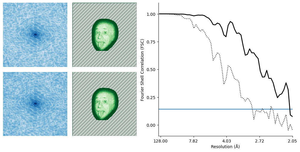
This is an underestimate of the true reliability of our reconstruction, because it includes noise from regions of space in which there is zero signal. We can instead calculate a *masked* FSC, in which we first mask each half map, then calculate an FSC between these masked half maps.

The region outside the mask (i.e., where the mask is set to 0.0) is hatched with white.

The masked FSC (solid) is markedly improved from the unmasked FSC (dotted), reflecting the fact that the region of the map we *expect to be correlated* is in fact well correlated. CryoSPARC actually calculates multiple masks and displays curves for each of them. More information about CryoSPARC’s FSC plots is available in [Tutorial: Common CryoSPARC Plots](https://guide.cryosparc.com/processing-data/tutorials-and-case-studies/tutorial-common-cryosparc-plots), and more information about automatic mask generation is available in [3D Masking in Refinement](https://guide.cryosparc.com/processing-data/tutorials-and-case-studies/tutorial-dynamic-masking-in-refinements-v5.0). ### Noise substitution It’s important to note here that the region outside the mask is set to zero, and so correlates perfectly. Thus, if we choose a small, detailed mask we can create an artificially high FSC.

None of the features visible in the masked map (the two eyes and the smile) are present in the unmasked map. However, because the vast majority of the box is set to 0 by the mask (and the non-zero regions are in exactly the same place), the map has a good FSC curve. Thus, by GSFSC alone, these mask artifacts appear to be reliable map features. To help reduce the effect of masking artifacts on the FSC curve, most cryo-EM refinement software packages calculate *noise-substituted FSC curves* at the end of a refinement (Chen et al. 2013). First, the phases of every Fourier component in the map beyond a certain resolution. In CryoSPARC, phases are randomized starting with the unmasked GSFSC resolution, or 75% of the masked GSFSC resolution, whichever is coarser. These phase-randomized half maps should have zero correlation in frequency shells with randomized phases.

In this example, phases are randomized starting with the unmasked GSFSC resolution (dotted vertical line). Note that, in Fourier space (blue), the maps become random noise starting at the corresponding distance from the origin.

Next, the mask is applied to these phase-randomized half maps.The tighter and more detailed the mask, the greater the introduced, artifactual correlation between the two half maps. In this case, because the mask is so small and detailed, the phase-randomized half maps correlate well until almost Nyquist.

Now that we know the level of correlation introduced solely by the mask, we can correct the masked GSFSC, attempting to remove this artifactual correlation. Because the low frequencies were not phase randomized, this correction is only performed beginning with the first randomized frequency shell. This produces the corrected GSFSC curve, which ideally tracks the tight mask GSFSC curve. In this case, because essentially all of the high-frequency correlation was induced by our mask, the corrected GSFSC immediately jumps to 0.

Compare this corrected curve to that of the loose mask, which in this case is a simple shape surrounding Einstein’s face.

Because the mask does not introduce significant bias at the relevant frequencies, the phase-randomized half-maps are essentially uncorrelated. Thus, the corrected curve tracks the masked curve closely, indicating that the GSFSC resolution estimate is not significantly biased by the mask. {% hint style="warning" %} CryoSPARC only performs this phase-randomization procedure at the end of the refinement, not during every iteration. The corrected FSC curve therefore indicates *only* whether the mask introduced bias *on its own*. A map with a corrected GSFSC curve that closely tracks the tight mask curve may still have noise that was overfit for other reasons. {% endhint %} ## GSFSC is a Global Measure Each Fourier shell considers signal at a given frequency in all directions, across the entire map. This comes with two important considerations. First, consider a particle stack in which all viewing directions except a select few are well sampled. This produces half maps with high correlation everywhere except a narrow band of each shell in Fourier space, so the overall GSFSC curve remains high even if the map itself becomes unusable. A concrete example of this can be seen in the case of [HA Trimer](https://guide.cryosparc.com/processing-data/tutorials-and-case-studies/case-study-picking-induced-orientation-bias-in-ha-trimer-empiar-10096-and-10097#missing-views-and-anisotropy), and this problem can be addressed with the [Orientation Diagnostics](https://guide.cryosparc.com/processing-data/all-job-types-in-cryosparc/utilities/job-orientation-diagnostics) job. Second, consider a map in which most of the particle is well-resolved, but a large flexible domain blurs out due to poor alignment. This blurry region has poor correlation between the half maps. Although this poor correlation is localized in *real* space, it is spread throughout all of *Fourier* space, and so hurts the entire GSFSC curve. This affects not only the resolution estimate, but also the filter applied at each iteration of a refinement, potentially limiting the quality of even the well-aligned, stable part of the target. A concrete example of this issue can be seen with [the yeast spliceosome](https://guide.cryosparc.com/processing-data/tutorials-and-case-studies/case-study-yeast-u4-u6.u5-tri-snrnp#global-refinement). The global impact of a poorly-aligned region can be attenuated by either providing a [resolution mask](https://guide.cryosparc.com/processing-data/tutorials-and-case-studies/tutorial-dynamic-masking-in-refinements-v5.0#masking-during-refinement) during the refinement, or by using [Non-Uniform Refinement](https://guide.cryosparc.com/processing-data/all-job-types-in-cryosparc/3d-refinement/job-non-uniform-refinement-new). ## Always Inspect Your Maps Although the GSFSC is a useful tool both to prevent overfitting and to provide a summary of a map’s overall quality, it is always essential to evaluate maps by manual inspection. The GSFSC is just one metric, and cannot measure the quality of particular regions of interest, or how two maps may differ in their overall interpretability. Maps should always be downloaded and manually inspected before moving on to downstream analysis steps. ## References Chen, S. *et al.* High-resolution noise substitution to measure overfitting and validate resolution in 3D structure determination by single particle electron cryomicroscopy. *Ultramicroscopy* **135**, 24–35 (2013). Harauz, G. & van Heel, M. Exact filters for general geometry three dimensional reconstruction. *Optik.* **73**, 146–156 (1986). Henderson, R. Avoiding the pitfalls of single particle cryo-electron microscopy: Einstein from noise. *Proceedings of the National Academy of Sciences* **110**, 18037–18041 (2013). Rohou, A. Fourier shell correlation criteria for local resolution estimation. *bioRxiv* 2020.03.01.972067 (2020) doi:[10.1101/2020.03.01.972067](https://doi.org/10.1101/2020.03.01.972067). Rosenthal, P. B. & Henderson, R. Optimal Determination of Particle Orientation, Absolute Hand, and Contrast Loss in Single-particle Electron Cryomicroscopy. *Journal of Molecular Biology* **333**, 721–745 (2003). Scheres, S. H. W. & Chen, S. Prevention of overfitting in cryo-EM structure determination. *Nature Methods* **9**, 853–854 (2012).