Job: Patch Motion Correction

At a Glance

Model full-frame and anisotropic motion in movies, and apply dose weighting, to produce motion-corrected micrographs.

Description

During movie collection, complex 3D deformations of the ice occur. When projected into a flat image, these 3D deformations appear as anisotropic motions of the ice, in which different regions of the image move in different directions. See e.g., (Thorne, 2020) for more details about the mechanism of anisotropic beam-induced motion.

Patch Motion Correction models this anisotropy by tiling a movie into patches and estimating the displacement of each patch in each frame under a motion model that is smooth over both space and time. It then corrects for the estimated motion by shifting each pixel based on its modeled displacement in each frame. Similar approaches are used in software such as MotionCor2 (Zheng et al. 2017) and Warp (Tegunov et al. 2018). Patch motion correction also applies Dose Weighting.

Inputs

Movies

This job requires raw movies in .mrc , .tif , .eer, or .mrc.bz2 format, typically from an Import Movies job.

Commonly Adjusted Parameters

Only process this many movies

This parameter selects the first n movies to process, rather than the entire input stack. It is most useful when working with a subset of movies to assess data quality before committing to a full processing pipeline.

If collection parameters changed during the collection, it may be better to use the Exposure Sets Tool job to select a random subset instead.

Low-memory mode

Reading movie files from disk is slow. To speed up processing, motion correction jobs process one movie and load the next simultaneously. However, this can lead to GPUs with low memory (i.e., < 16 GB VRAM) to run out of memory. Turning this option on causes the job to wait to load the next movie until it has finished processing the current movie. This slows down the job, but can prevent out-of-memory errors.

Save results in 16-bit floating point

Save the output micrographs in 16-bit floating point. We recommend that this option is turned on to save space at minimal loss of accuracy. See the 16-bit floating point article for more information.

Output denoiser training data

When this parameter is turned on, Patch Motion Correction will produce the even and odd half-micrographs necessary to train the Micrograph Denoiser. Note that these half-micrographs do take up a small amount of disk space — the training data pair takes up as much space as the motion-corrected micrograph. For a 4k frame saved in 16-bit format, the default 200 movie training set takes up approximately 12 GB of disk space.

Num. movies for denoiser training data

This parameter sets the number of movies for which denoiser training data is produced and defaults to 200. Generally, 100 micrographs are sufficient to train the denoiser. By default, more training data is produced in case some micrographs with training data are excluded in, e.g., a Curate Exposures job. If space is a significant concern, or if no micrographs will be excluded before training the denoiser, this parameter can be reduced to the number of micrographs you plan to use when training the denoiser.

Output F-crop factor:

Reduce the size of the output, aligned micrographs by this factor. If the F-crop (Fourier-crop) factor is 1.0, no cropping is performed. A crop factor of 0.5 downsamples output micrographs by half, discarding the highest-frequency half of the Fourier components, etc. This significantly reduces the file size of the final micrographs, but limits the maximum resolution possible for resulting reconstructions.

Particle images can also be Fourier-cropped (downsampled) at the Extract from Micrographs stage. It is often common to initially process downsampled particle images (to speed up particle curation and early reconstructions) and then return to full resolution particle images downstream in final refinements. This type of workflow is made easier if the motion corrected micrographs are not downsampled, and the downsampling is instead only applied at the extraction stage. As such, for a general workflow and non-super-resolution movies, we recommend using the default Output F-crop factor of 1.0 during motion correction. When working with super-resolution movies, we recommend downsampling to the physical detector pixel size (i.e., setting Output F-crop factor to 0.5 for 2x super-resolution movies). Of course, there are some datasets that benefit from the full, super-resolution pixel size, and some which benefit from more aggressive downsampling.

Start frame and End frame

These parameters allow discarding frames from the start and end of the input movies, before motion correction is applied. This can be helpful in case there are artefacts or issues with early or late frames. For example, some cameras can have issues where they output one or more blank frames at the end of a movie, and these can disturb motion estimation.

Override knots X

Spline knots control the smoothness of motion trajectories that will be optimized by Patch motion correction (see Method Details below). CryoSPARC automatically determines the number of knots in each spatial and temporal direction based on characteristics of the input movies (e.g., magnification, dose rate, etc) and it is not generally necessary to change these parameters. These parameters can be used to enforce additional smoothness on motion trajectories (setting knots to a low value) or allow patch motion correction to model additional anisotropy (setting knots to a high value) beyond its automatic settings, if needed.

Importantly, the knot parameters do not change the number of patches or size of patches used by Patch Motion Correction. Patches are 500 Å wide and cannot be resized by the user.

Outputs

Micrographs

Aligned micrographs for further downstream preprocessing. These micrographs also have rigid motion estimates, which are required for jobs like Reference-Based Motion Correction and Local Motion Correction.

Micrographs incomplete

Micrographs which were not successfully corrected are output in this group. Typically this is due to some error specific to the movie — the Event Log should contain more information on why a particular movie failed.

Common Next Steps

Typically, micrographs must have their CTF estimated, via e.g., Patch CTF Estimation, before any further processing can occur.

Method Details

Patch Motion Correction progresses through three main steps for each movie: rigid motion estimation, anisotropic motion estimation, and motion correction.

Rigid motion is estimated in much the same way as Full-Frame Motion Correction. More detail is available in that article, but in short, a full-frame trajectory is iteratively optimized to produce the highest degree of correlation between all frames.

An example micrograph from EMPIAR 10674.

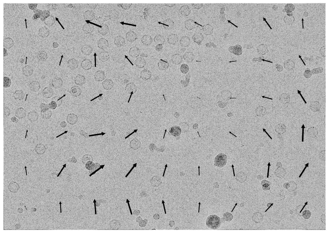
Next, the micrograph is split into overlapping 500 Å patches. In order to model anisotropic motion (i.e. deformation of the sample), the motion trajectories of all patches are jointly optimized to produce the highest degree of correlation across all frames of the movie. In this optimization setup, for each patch, each frame (denoted by a Z dimension representing time) is allowed to shift in both X and Y directions.

An example of a single frame’s patch displacement. An arrow represents the displacement of a patch in a single frame. Note that the length of the arrows are scaled for visibility.

The optimization of patch trajectories is constrained using a spline function. The number of knots (i.e. degrees of freedom) in the spline function is automatically selected by CryoSPARC based on the magnification and dose rate of the input movies, and the spline serves to restrict the possible patch trajectories that the optimization can model to ensure that they are smooth over both space and time. Furthermore, after optimization, the spline function allows interpolation of displacement for each pixel, rather than only at the patch level.

X and Y displacement models for a single frame are shown with pink and blue surfaces, respectively. Using this function, each pixel’s displacement can be modeled.

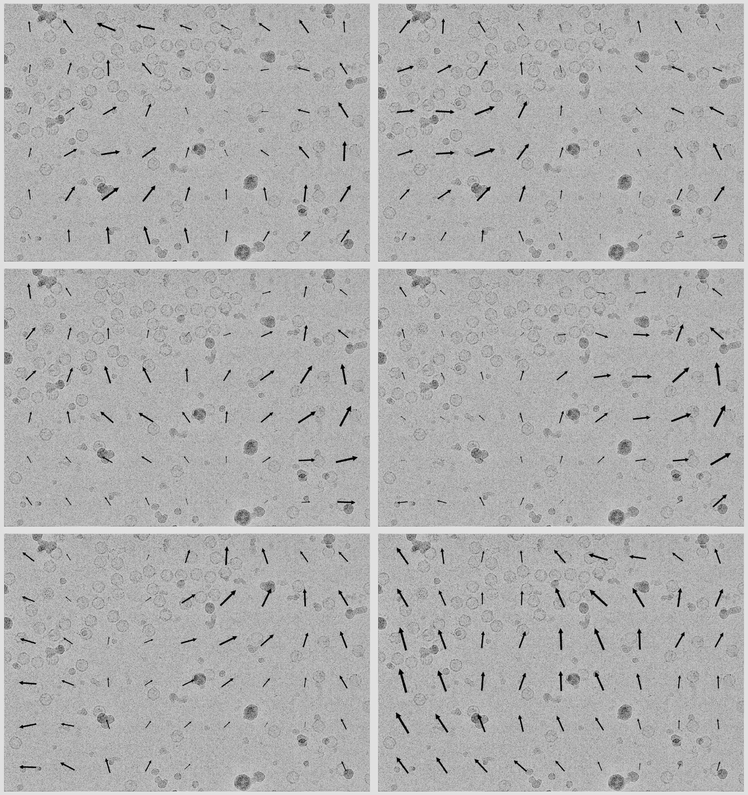
As mentioned, the number of spline knots control the number of degrees of freedom used by the motion model in each of the three dimensions (X, Y, and time). A small number of knots causes the model to be smooth, which protects from overfitting but may also prevent the spline functions from fully capturing the dynamics of patch movement. A large number can have the opposite effect. CryoSPARC automatically selects the number of knots.

The full motion model, optimized using data across all frames, provides an estimate of the anisotropic motion during the entire movie:

which in turn can be used to model each pixel’s trajectory through time and space:

Each pixel’s displacement varies as it moves through time, and so do the spline functions.

After motion estimation, the final spline function provides the optimal prediction of the shift of any given pixel for each frame. This prediction is used to shift each pixel in each frame by the modeled displacement to produce a single, motion corrected averaged micrograph from which particles can be picked and extracted. Note that this is distinct from other motion correction jobs, like Local Motion Correction, that model and correct the motion of individual particles and produce extracted particles rather than a complete micrograph.

Example Workflow

Tutorial: Patch Motion and Patch CTF

References

1. Robert Thorne, “Hypothesis for a Mechanism of Beam-Induced Motion in Cryo-Electron Microscopy,” IUCrJ, 2020, https://doi.org/10.1107/S2052252520002560.

2. Zheng, S. Q. et al. MotionCor2: anisotropic correction of beam-induced motion for improved cryo-electron microscopy. Nature Methods 14, 331–332 (2017).

3. Tegunov, D. & Cramer, P. Real-time cryo-EM data pre-processing with Warp. bioRxiv (2018) doi:10.1038/s41592-019-0580-y.