Get Started with CryoSPARC: Introductory Tutorial (v4.0+)
In this tutorial, we will process a small dataset from movies to reconstructed density map. If you are new to data processing in CryoSPARC, we highly recommend following along!
Last updated
In this tutorial, we will process a small dataset from movies to reconstructed density map. If you are new to data processing in CryoSPARC, we highly recommend following along!
Last updated
The information in this section applies to CryoSPARC v4.0+. For CryoSPARC ≤v3.3, please see: Get Started with CryoSPARC: Introductory Tutorial (v3)
We recommend starting off with the T20S Tutorial to become familiar with the workflow in CryoSPARC. When you're ready to learn more about cryoEM, you might move on to or other .
This dataset is a subset of 20 movies from the T20S Proteasome dataset. While not a representative example of the complexity of most cryo-EM projects today, it is a good way to become familiar with the interface and software features and to .
For a refresher on the interface, projects and jobs, please see the .
CryoSPARC organizes your workflow by Project, e.g, P1, P2, etc. Projects contain one or more Workspaces, which in turn house Jobs.
Projects are strict divisions. Files and jobs from different projects are stored in dedicated project directories and jobs cannot be connected from one project to another.
Workspaces are soft divisions, and allow for logical separation of jobs and workflows so they can be more easily managed in a large project. Jobs may be connected across workspaces and each job may belong to more than one Workspace.
To create a project, click on the New Project button at the top right side of the header.
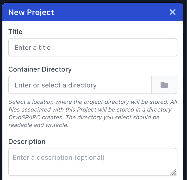
A dialog box will open to the right, prompting you for a project title, container directory, and optionally a description.
Enter a project title and browse for a location for the associated container directory with the file browser. The container directory should already exist. CryoSPARC will create a subdirectory within the container directory that will become the project directory for the new project, and will act as a root for all new files and directories created in the project. This includes job directories, imported jobs and result groups, and exported jobs and result groups.
You may also enter a description for your project.
Click Create. The new project now appears on the Projects page, accessible via the container icon on the navigation bar.
Use Workspaces to organize or separate portions of the cryo-EM workflow for convenience or experimentation. Create at least one Workspace within a Project before running a Job.
After creating a new project, you will be prompted to create a new workspace within the project. Enter a title, such as "T20S Subset Processing", and click Create Workspace. Note that both the title and description can be modified later.
If you have exited the project view, you can always navigate back to it by clicking the container icon on the navigation bar, then clicking anywhere on your newly created project card (in this example, P35), and finally selecting View Project on the right-hand sidebar. The container icon and the View Project button are highlighted in purple boxes in the image below. Projects can also be navigated to using the search functionality, accessible via the magnifying glass in the lower left corner of the interface:
Once within the project, new workspaces can also be created at any time using the New Workspace button at the top right side of the header.
Log in to the machine where CryoSPARC is installed via command-line.
Run the command cryosparcm downloadtest
while in this directory. This downloads a subset of the T20S dataset.
Run tar -xf empiar_10025_subset.tar
to decompress the downloaded data.
In CryoSPARC, navigate to the new Workspace. To do so, navigate to the project as described in step 2, then click on the workspace card, and hit View Workspace on the bottom right.
Select the Movies data path: Click the file browse icon and select the movie files (.mrc
or .tif
format). To select multiple files, use a wildcard, e.g., *.mrc
. This selects all files that match the wildcard expression. The file browser displays the list of selected files along with the number of matches at the bottom. For this tutorial dataset, navigate to the directory where the test data was downloaded. Use the wildcard expression *.tif
to select all TIFF format movies in the folder. There should be 20 imported movies.
Select the Gain reference path with the file browser: Select the single .mrc
file in the folder where the test data was downloaded.
Raw pixel size (Å): 0.6575
Accelerating voltage (kV): 300
Spherical abberation (mm): 2.7
Total exposure dose (e/Å^2): 53
After changing a parameter, the parameter box and title changes colour from gray to green. This indicates the parameter is different from its default value:
Click Queue Job to start the import. Use the subsequent dialog to select a lane/node on which to run the job. The available lanes depend on your installation configuration. By default, import and interactive jobs will run on the master node as they are not resource intensive. Using this dialog box, you may set the job title and description, which may both be changed later. Press the Queue button.
The Import Movies job queues and starts running. Look for the Job card in the workspace to monitor its status.
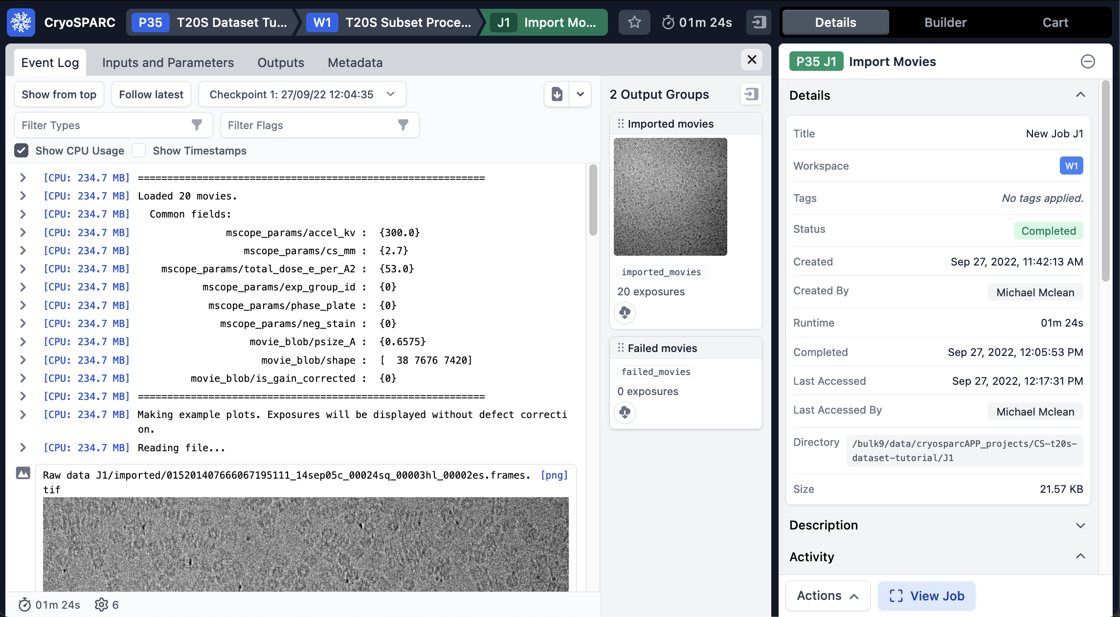
To open a Job and view its progress, click on the header at the top of the Job card, where the job title is shown. Alternatively, select on the Job card and press the spacebar on your keyboard:
To exit the job/close the inspect view, press the spacebar again, or press the ×
button on the top-right of the dialog.
Once finished, the job's status indicator at the top left changes to "Completed" in green.
The Patch Motion Correction job requires raw movies as Inputs. First, ensure that the Patch Motion Correction job is in Building status. Open the previously completed Import Movies job by clicking on the header of the job card, then drag and drop the Outputs of the Import Movies job, to the Movies placeholder in the Job Builder.
Once dropped, the connected output name appears in the Job Builder as an Input:
If you have multiple GPUs available, you can speed up the processing time by setting the Number of GPUs to parallelize parameter within the Compute settings section to the number of GPUs you would like to assign to that job.
Queue the job and select a lane. It is generally not necessary to adjust the Patch Motion Correction job parameters; they are automatically tuned based on the data. Finally, click Queue.
Once the job starts to run the card will update with a preview image:
This job type requires micrographs as the input. Open the previous Patch Motion Correction job, and drag and drop the output (20 micrographs) into the Micrograph placeholder in the Job Builder.
As with Patch Motion Correction, the job will complete faster by allocating multiple GPUs. This can be configured with the Number of GPUs to parallelize parameter.
Queue the job to start. It is generally not necessary to adjust the Patch CTF Estimation job parameters; they are automatically tuned based on the data.
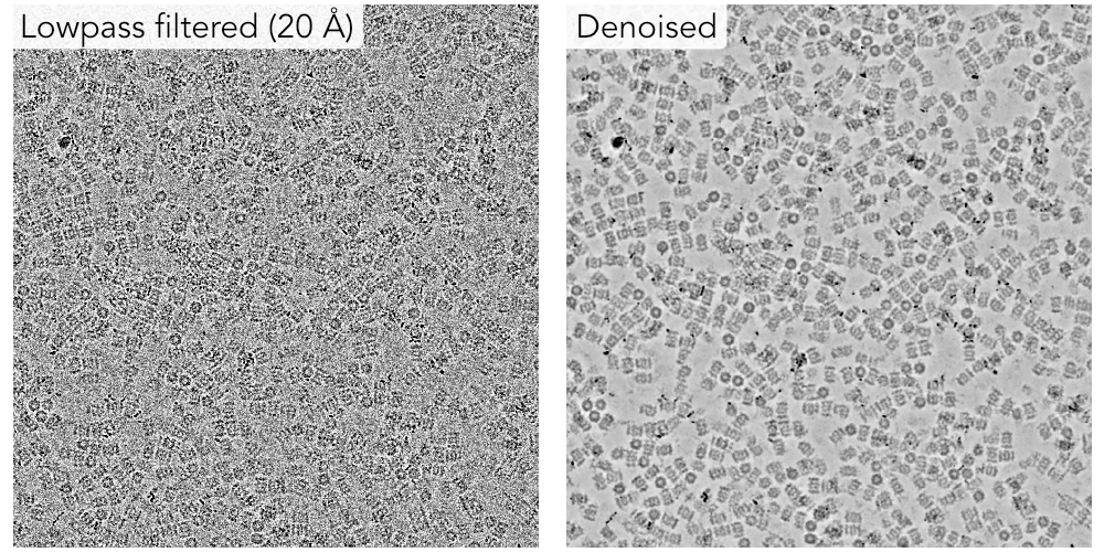
The motion-corrected micrographs now have CTF estimates. The next step of the Single Particle Analysis pipeline is picking particles, in which each micrograph is scanned for positions which are likely to contain a particle ("picks"). However, cryo-EM micrographs often have very poor signal-to-noise ratio. This makes visual inspection of micrographs difficult, and also makes particle picking difficult, resulting in many off-target picks.
Select Micrograph Denoiser in the Job Builder to create a job
Open the previous Patch CTF Estimation job and drag the Micrographs processed output to the exposures input.
Leave the optional Denoise model input empty, as we have not yet trained a model on this dataset.
Typically, the parameters of Micrograph Denoiser can be left as default. However, since this dataset contains fewer than the default 100 micrographs used for training, we must adjust the Number of mics for training parameter to 20
.
Queue the job to start.
To create the Blob Picker job using Quick Actions, move your cursor over to the Micrograph Denoiser job card and click on the ellipsis (...) in the header of the job card. Alternatively, right click anywhere on the job card.
Scroll down and click on the Build Blob Picker on Denoised Mics button. This will create the Blob Picker job and connect the output Denoised micrographs from the Micrograph Denoiser job to the Blob Picker job, all in one click.
If you did not use the Micrograph Denoiser, select the Build Blob Picker option from the Quick Actions of the Patch CTF Estimation job instead.
Once built, enter the Job Builder of the Blob Picker job on the right sidebar, and set Min. Particle Diameter to 100
and Max Particle Diameter to 200
.
If you are using denoised micrographs, ensure that Pick on denoised micrographs is turned on.
Some contaminants, like carbon support or crystalline ice, are often labeled with many particle picks due to their high contrast. These off-target picks ("junk picks") degrade performance of downstream analysis and should be removed. The Micrograph Junk Detector analyzes the input micrographs and annotates each micrograph with the location of various common types of junk and then removes particle picks from those locations.
Select Micrograph Junk Detector from the Job Builder.
Open the previous Blob Picker job.
Drag the Micrographs output from Blob Picker into the Exposures input of the Micrograph Junk Detector builder.
Drag the All particles output from Blob Picker into the Particles input of the Micrograph Junk Detector builder.
Leave all parameters at their default values and launch the job.
The Micrograph Junk Detector produces diagnostic plots for the first 20 micrographs (which, for this dataset, is all of them). These plots show which regions of the micrograph have been marked as junk, as well as indicating which particles have been rejected because they are too close to junk.
Select Inspect Particle Picks from the Job Builder, or by using Quick Actions from the previous Micrograph Denoiser job.
Once the previous Micrograph Denoiser job has completed, drag and drop both the Particles accepted and Labelled micrographs outputs from the previously completed Micrograph Denoiser job. Queue the job.
Once the job is ready to interact with, it will be marked as "Waiting" and an "Interactive" tab will be available in the job details dialog:
The left side of the interactive tab shows three sections. From top to bottom:
The Exposure Plot displays a customizable scatter plot, allowing various statistics of the exposure dataset (e.g. number of picked particles, average defocus, etc.) to be plotted against each other.
Below the Exposure Plot is the Power Histogram, which displays a 2D histogram of all picked particles. The y-axis measures the Power Score, and the x-axis measures the Normalized Cross-Correlation (NCC) Score for each particle pick. Note that the histogram includes both true particles, as well as false positives that were picked up during the blob picking. True particles generally have high NCC scores (indicating agreement in shape with the templates) and a moderate-to-high Power score (indicating the presence of significant signal). Picks that have too little power are false positives containing only ice, while picks with very high power are carbon edges, ice crystals, aggregate particles, etc.
Finally, the Micrographs tab displays a list of each micrograph in the dataset, along with some statistics for each micrograph. Any micrograph row can be clicked on, to display it on the right panel along with the selected particle picks in green circles.
Make adjustments to the parameters below if needed. All adjustments are saved automatically. As parameters are adjusted, the selected particle picks on the displayed micrograph will be simultaneously updated.
Adjust the Particle Diameter to make it easier to see the location of picks.
Clicking the vertical ellipsis button on the top right allows for selection of colours, and whether to display the denoised micrograph or raw micrograph.
If viewing raw micrographs, move your cursor over the micrograph display, and adjust the lowpass filter slider if needed to better view the picks. It may be easier to view the particles at a lowpass filter value between 20 to 30 Å.
Slowly increase the NCC slider and watch the particle pick locations on the right. Keep increasing it until empty ice picks stop disappearing and good particles begin to disappear, then reduce it to just below that point. For this example, with denoised micrographs, this value was around 0.41
.
If any picks on empty ice remain, slowly increase the lower Power threshold slider until the empty ice picks are removed, but without removing any good particles to do so.
If any picks remain on high-contrast contaminants, slowly reduce the higher Power threshold slider until these junk picks are removed, but without removing any good particles to do so.
Once satisfied with the picks, select "Done Picking | Output Locations" button. This completes the Inspect Particle Picks job and saves selected particle locations.
This job extracts particles from micrographs, and writes them out to disk for downstream jobs to read.
Open the recently-completed Inspect Picks job. Drag and drop both the Micrographs accepted and Particles accepted outputs into the corresponding inputs on the Job Builder.
In the Job Builder, look under the Particle Extraction section and change the Extraction box size (pix) to 440
. You may also parallelize the Extract From Micrographs over multiple CPU cores by altering the Number of CPU cores parameter, under Compute settings.
Queue the job.
Once the job completes, you'll notice the number of resulting particles is less than the input; this is due to the fact that particle extraction process excludes picks that are too close to the edge of the micrograph:
Drag and drop the Particles extracted output from the previously completed Extract from Micrographs, into the input and queue the job.
In the event log, preview images of class averages appear after each iteration. Classification into 50 classes (the default number) takes about 15 minutes on a single GPU.
The quality of classes depends on the quality of input particles. While we could use these blob-picked particles directly for 3D Reconstruction, we can obtain better results by repeating our particle picking using these templates generated by 2D Classification. Thus, in this tutorial, we will use these classes to inform the Template Picker of the shape of our target structure. The next step in this workflow is the Select 2D Classes job.
Drag and drop both the All particles and 2D class averages outputs from the most recently completed 2D Classification job.
Queue the job. Once the data is loaded, the job status changes to Waiting and Interactive class selection mode is ready.
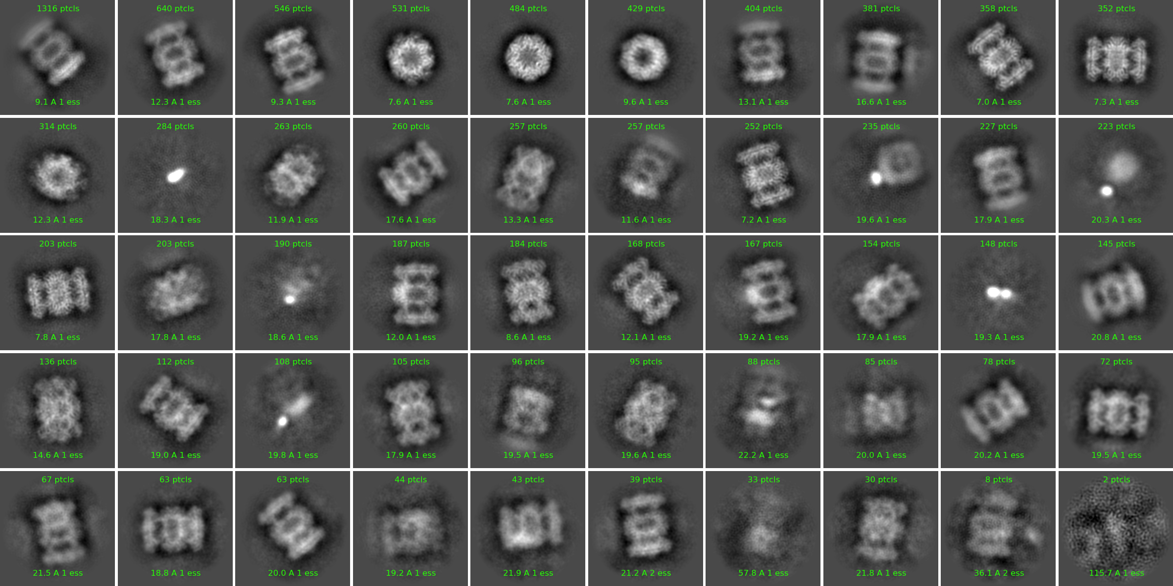
Select a "good" class for each distinct view of the structure. In this case, a top view and side view are the most common views present in the dataset. Use both the number of particles and the provided class resolution score to identify good classes of particles. The interactive job provides several ways to sort the classes in ascending or descending order based on:
# of particles: The total number of particles in each class
Resolution: The relative resolution of all particles in the class (Å)
ECA: Effective classes assigned. Classes with a higher ECA value have less confident particle assignments.
Use the sort and selection controls to quickly sort and filter the class selection. Each class has a right-click context menu that allows for selecting a set of classes above or below a particular criteria.
Avoid selecting classes that contain only a partial particle or a non-particle junk image when creating templates, since these will result in off-center particle picks.
When finished, select Done at the top right side of the window. The job completes.
Create the Template Picker job using the Job Builder.
Connect the Templates selected output of the Select 2D into the template input
Connect the Micrographs processed output of the Patch CTF Estimation job into the micrographs input
Set the Particle diameter (Å) value to 190
Queue the job. It should take around 15 seconds to process the dataset.
As with the Blob Picker, use the Inspect picks job to view and interactively adjust the results of template-based automatic particle picking.
Select Inspect Particle Picks from the Job Builder, or by using Quick Actions from the previously completed Template Picker job.
Drag and drop both the All particles and micrographs outputs from the previously completed Template Picker job. Queue the job.
Set the NCC and Power thresholds using the same process as the previous Inspect Picks job. Slowly increase the NCC score until good particles start disappearing, then adjust the power scores as necessary.
Click Done Picking | Output Locations to complete the job as before.
We will now repeat the extraction process given the new set of pick locations generated by the latest Inspect Picks job.
Open the recently-completed Inspect Picks job. Drag and drop both the micrographs and All particles outputs into the corresponding inputs on the Job Builder.
In the Job Builder, look under the Particle Extraction section and change the Extraction box size (pix) to 440
.
Select 2D Classification from the Job Builder.
Drag and drop the particles extracted output from the previously completed Extract from Micrographs, into the input and queue the job.
The particles extracted from the template picker result in much higher quality 2D classes. Proceed to the next step to filter out the highest quality classes for 3D reconstruction.
Select Select 2D Classes from the Job Builder.
Drag and drop both the All particles and 2D class averages outputs from the most recently completed 2D Classification job.
Once queued and running, switch to the Interactive tab and select all of the good quality classes.
In this case, we want to keep all true particles in our dataset (rather than just selecting one top and one side view, as previously done in step 11), and reject all false positives.
The visual quality of a 2D class, together with its resolution, number of particles, and ECA, can all provide proxy measurements of the quality of the underlying particles that comprise the class.
Note that clear "junk" classes, corresponding to non-particle images, ice crystals, etc., should be rejected at this stage. Err on the side of keeping a 2D class — when a class looks like a blurry version of the particle, it should be kept at this stage. For example, the following shows one possible selection of 2D classes to retain:
Once clicking Done, the job will generate outputs for each group of classes and particles, one for the selected set and another for the excluded set:
Drag and drop the Particles selected output from the most recently completed Select 2D classes job (classes selected from the result of the template picker) into the Particle stacks input in the Job Builder.
Note: You do not need to enforce symmetry during Ab-initio Reconstruction.
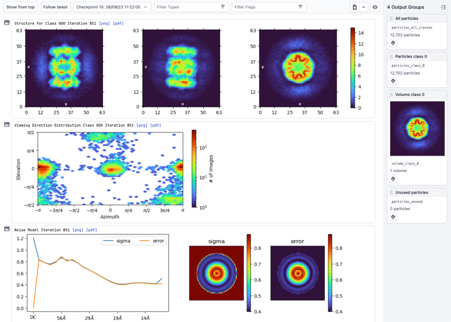
Queue the job. Results appear in real-time in the event log as iterations progress. Ab-initio reconstruction should generate a 3D density of the T20S structure at a coarse resolution, with no initial model required.
Select Homogeneous Refinement from the Job Builder.
Drag and drop both the All particles and Volume class 0 from the recently completed Ab-initio Reconstruction into the Particle Stacks and Initial Volume inputs, respectively. Leave the Static mask input empty.
Set the following parameter:
Symmetry: D7
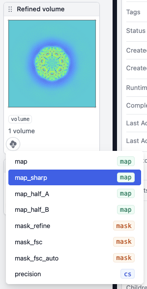
Once complete, download the volume and/or mask directly from the Outputs section on the right hand side: Select the drop-down to choose the outputs you wish to download. A refinement job outputs a map_sharp
, the final refined volume with automatic B-factor sharpening applied and filtered to the estimated FSC resolution.
CryoSPARC automatically generates masks for FSC calculation. However, it is generally good practice to generate your own FSC mask to ensure the calculation is repeatable across jobs, and to ensure the mask covers the entire relevant region of the protein.
First, use Volume Tools to lowpass filter the refined volume. This step is important because masks themselves should generally be smooth to avoid introducing bias.
Set the Lowpass filter (A) value to 10
.
Launch the job.
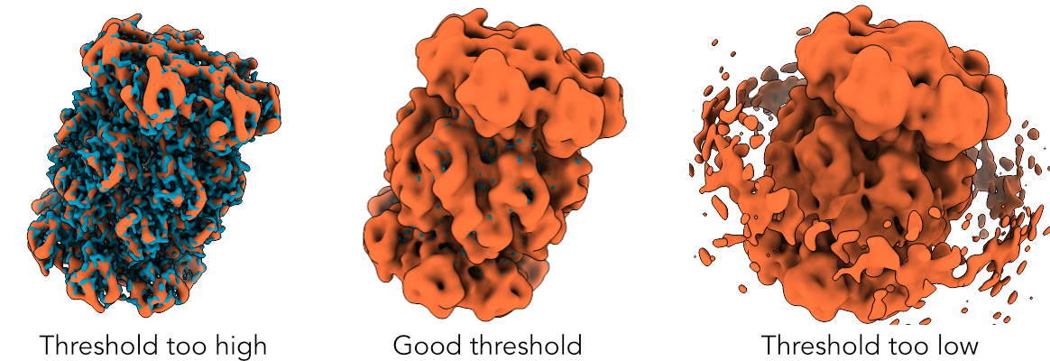
This job lowpass filters the volume, producing a smoothed version suitable for mask creation. Download and inspect the smoothed map in ChimeraX. Find the highest threshold for which no noise is visible in the smoothed map.
Create another Volume Tools job and connect the Volume output of the previous Volume Tools job to the Input volume input.
Set Type of output volume to mask
.
Set Threshold to the value you found in ChimeraX.
Set the Dilation radius (pix) to 4
. This ensures that all information from the map is contained in the mask.
Set the Soft padding width (pix) to 14
. It is important that all masks in CryoSPARC have soft padding added to avoid artifacts.
Launch the job.
This job creates a mask which can be used in an Validation (FSC) job.
Connect the Refined volume output from Homogeneous Refinement to the Input volume input.
Connect the Mask output from the second Volume Tools job to the Static mask input.
Set Compute facility to GPU
.
Launch the job.
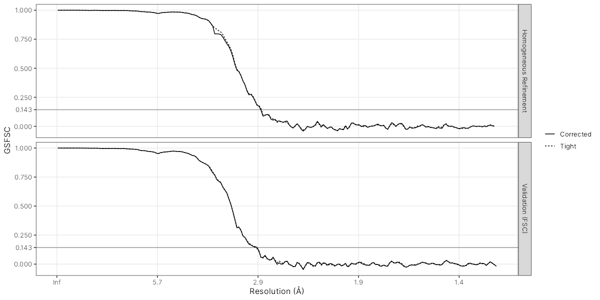
This job produces similar outputs to the GSFSC plots produced by Homogeneous Refinement, but provides better control over the mask used to calculate the GSFSC and allows for repeatable, directly-comparable analysis of resolution.
For optimal results in publications and for model-building, it is often necessary to re-sharpen and adjust the B-factor. This step is optional as Homogeneous Refinement already outputs a sharpened volume (map_sharp
) with a B-factor reported within the Guinier plot.
Drag and drop the volume output from the result of the previous refinement job, into the volume input.
Set a B-Factor. Get a good starting B-Factor value from the final Guinier plot in the stream log of the refinement job you previously ran. It is recommended to input a B-Factor (as a negative value) ±20 the reported value in the plot. In this case, -56.7
and -96.7
Activate the Generate new FSC mask parameter, which will generate a new mask for the purposes of FSC calculation from the input volume. This is done by thresholding, dilating, and padding the input structure.
Queue the job. Once complete, download the sharpened map (map_sharp
) from the output.
After visually assessing the map, optionally run another sharpening job (clear or clone the existing one) with a different B-Factor.
Now that you have refined the data to a high-resolution structure, you can apply more advanced processing techniques. Explore the job builder and other documentation to see the available job types and processing options. Common workflows include:
Sub-classification to identify small, slightly differing populations
Re-pick with multiple higher quality 2D classes
For detailed explanations on all available job types and commonly adjusted parameters, see:
Check back to see updates to this guide, as new features and algorithms are in constant development within CryoSPARC.
The Dashboard provides at-a-glance information on currently active jobs, and your instance's processing history. It also displays links to various resources, including the , , the , and recent entries from the and . As well, the dashboard displays the for new versions of CryoSPARC. The navigation bar on the left side of the UI contains links to the Projects view, the , , , job history, and more.
Navigate to or create a directory into which to download the test dataset (approx. 8 GB). This location should have read permissions for .
You will be greeted with a list of the various , with links to quickly build any of them. For this tutorial, we can get started with data processing by clicking to build an job.
This creates a new job within the current Workspace, displayed as a card. By default, new jobs are set to Building status, indicated on the job card in purple. To change parameters, select the job and ensure that the job is in Building status. A job's status can be , or by clicking the Build or Stop Building badges on the job card.
Edit Job parameters from the Builder; enter the following parameters (obtained from the original publication in ).
This opens the , which shows a streaming event log of the real-time progress for the Import Job. Scroll through the event log to view results. Select a checkpoint to find a specific location in the event log or click 'Show from top' to return to the beginning. Additional actions and detailed information for the job are available in the details panel. The Output of the import job, i.e., the 20 imported movies, are available on the right hand side of the event log:
For our next stage of processing, we will be performing on the imported movies. Motion Correction refers to the alignment and averaging of input movies into single-frame micrographs, for use downstream.
Select the in the right sidebar by clicking on the Builder tab. The Job Builder displays all available job types by category (e.g., workflows, imports, motion correction, etc.). A tutorial on the Job Builder and other ways to build jobs in CryoSPARC (Quick Actions, Job Cart) is available .
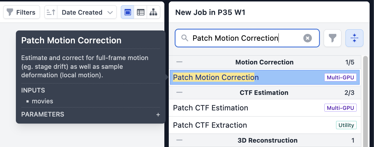
Select the job type in the Job builder. You can either scroll down and locate the job within the "Motion Correction" category, or you may search for it using the search tool. This creates a new job in building state so that its inputs and parameters are editable in the right side panel.
Our next step is to perform . This stage involves the estimation of several CTF parameters in the dataset, including the defocus and astigmatism of each micrograph.
Select in the Job Builder to create a new job.
You can connect outputs of jobs that haven't completed into the inputs of a building job. In this case, the newly created job will start to run automatically when all parent jobs have completed. This makes it easy to to run without having to wait until they're completed to queue them manually.
The is a trained neural network that learns to flatten the background noise and increase contrast in particles, making picking more effective. This typically improves performance of all picking techniques, increasing the number of correct particles found and reducing the number of false positives.
A denoiser model will be trained on all 20 micrographs of the dataset, and then automatically used to denoise the micrographs for downstream use. More information about how this job works and explanations of the various parameters are available in the .
It is important to attain a large number of high-quality particles for an optimal reconstruction. The is a common starting point for particle picking as it is a quick way to obtain an initial set of particle images that can be used to refine picking techniques over time.
Blob picking is a good idea because it verifies data quality and sets expectations for what particle images, projections, and structures should look like. We'll use blob picks to generate a set of templates that can be used as an input to the , which will generate a set of much higher-quality picks matching the two primary 2D views of the T20S structure.
For certain jobs, CryoSPARC has built-in . These are shortcuts that allow you to simultaneously build a downstream job while connecting an existing job's outputs to it, all in one step.
Use the job to view and interactively adjust the results of blob-based (and template-based) automatic particle picking.
Select in the Job Builder, or by using Quick Actions from the previously completed Inspect Picks job.
We generally recommend selecting a box size that is at least double the diameter of the particle. The box size controls how much of the micrograph is cropped around each particle location. Larger box sizes capture the most high-resolution signal that is spread out spatially due to the effect of defocus (CTF) in the microscope. However, larger box sizes significantly increase computation expense in further processing. To mitigate this, you can use the to speed up processing for jobs that do not require the full spectrum of data such as 2D Classification.
is a commonly used job in cryo-EM processing to get a first look at the data, group particles by 2D view, remove false positive picks, and even to get early insights into potential heterogeneity present in the dataset. In this step, we will use 2D Classification to group particles by 2D view, and then use the resulting class averages (also referred to as "templates") to improve our particle picking.
Select from the Job Builder, or by using Quick Actions.
allows us to select a subset of the generated templates from 2D Classification, and to reject the rest.
Select from the Job Builder, or by using Quick Actions.
The operates similarly to the Blob Picker but allows for an input set of templates to use to more precisely pick particles that match the shape of the target structure.
Select .
Now that we have a set of good quality particle picks, we can proceed into .
Select from the Job Builder.
Now that we have a low-resolution 3D density, we can the density to high-resolution using the job.
Queue the job. Results appear in real time in the stream log. The refinement job performs a rapid gold-standard refinement using the Expectation Maximization and branch-and-bound algorithms. The job displays the current the resolution, measured via , and other diagnostic information for each iteration.
Note that the GSFSC resolution is less than half of the Nyquist resolution for these particles. The particles could therefore be safely downsampled (using ) to speed up subsequent jobs with no loss in resolution.
More information on mask design and creation in CryoSPARC is available in the dedicate tutorial.
Create a job and connect the Refined volume output from the previous Homogeneous Refinement job to the Input volume input.
Create a job from the job builder.
Sharpen the result of the refinement with the from the Utilities section in the Job Builder.
Once you have assembled a workflow of connected jobs within a project, you can switch to the to understand how jobs are connected to obtain the final result. Click the flowchart icon in the top header:
Within the Tree View, you can select jobs and modify/connect them in the same way as previously demonstrated in the Card view. For more information on the Tree view and other useful tips, see the .
to explore both discrete and continuous heterogeneity in the dataset
to improve resolutions by accounting for disordered regions and local variations in a structure
or to refine multiple conformations and simultaneously classify particles
Heterogeneous to find multiple unexpected conformational states or multiple distinct particles in the data
Multiple rounds of to remove more junk particles
to focus on sub-regions of a structure
(per-exposure-group) or (per-particle)
cryoem2
lane.